Chapter 35 - Automated Data Processing for the Geological Atlas of the Western Canada Sedimentary Basin |
|
| Chapter Sections | Download |
Authors: I. Shetsen - Agis Associates Ltd., Edmonton
G.D. Mossop - Geological Survey of Canada, Calgary
Introduction
Atlas computing and data processing embrace a multitude of operations on hundreds of data files and thousands of data elements, and involve scores of activities, ranging from the development of analytical techniques and associated software to painstaking construction of various map layers. This chapter provides a brief description of the essential elements of Atlas data processing and mapping; there is simply no space here to enumerate and describe all the methods, operations and steps involved in the production of Atlas maps. Procedures and techniques of general applicability are to be published separately, in the open literature. Details of the organization of the elements in the Atlas database are set out in the documentation that accompanies the digital release of Atlas data.
Much of what is presented here is intended for readers who are conversant with computer data processing and the mathematical and statistical methods employed in computer data analysis, including pattern recognition approaches.
Scope and Constraints
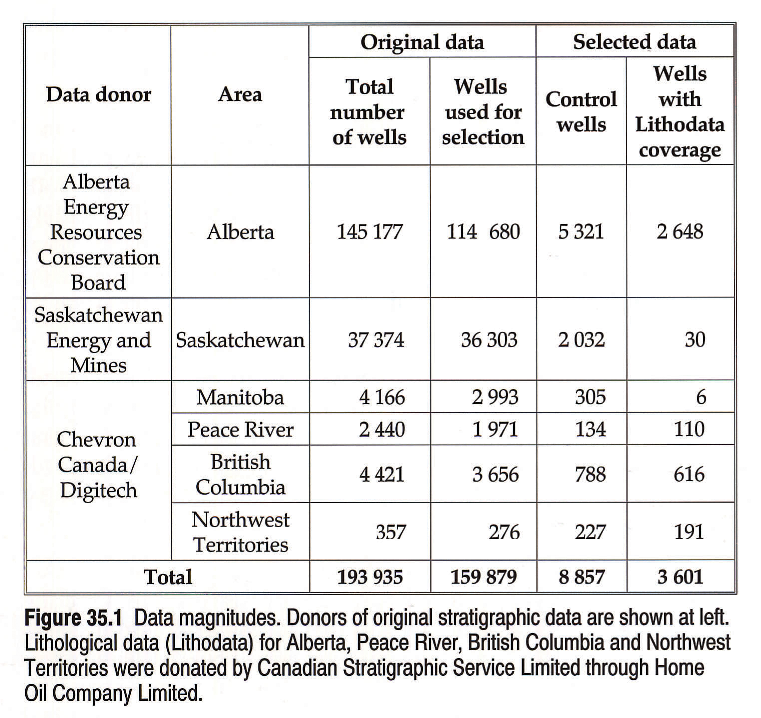
The Atlas mapping is based on voluminous digital subsurface data collected prior to 1987 and donated to the project by government agencies and private companies (Fig. 35.1). These databases contain comprehensive and systematic information on well stratigraphy and lithology, and provide exceptional to adequate control for virtually the entire Western Canada Sedimentary Basin. However, given the regional scale of Atlas mapping, utilization of the whole wealth of information poses several problems. The cost of converting vast volumes of records directly into map inputs and maps would be prohibitive. The density of drilling is uneven, and locally far exceeds the resolution of Atlas maps. The data contain a certain degree of redundancy and inconsistency, and require reassessment and culling prior to usage. To perform revisions on the scale of all of the original data would have been clearly beyond the available resources.
Consequently, the original data were evaluated, filtered and distilled into a manageable subset of approximately nine thousand Atlas control wells, selected on the basis of one representative well per township or equivalent area. To compensate for the inevitable loss of information induced by data reduction, the database was augmented by additional data sets, of both a generalized and a detailed nature, described below under Atlas Database.
The record of stratigraphic picks in Atlas control wells was substantially revised and refined by the chapter teams. The iterative process of database and map upgrading, outlined schematically in Figure 35.2, continued throughout the life of the project, using a combination of automated and manual data evaluation methods. The final Atlas maps, although compiled with considerable manual input, are an offspring of several generations of computer maps that were produced at project headquarters, and dispatched, together with accompanying computer-generated reports on data inadequacies, to chapter teams for review and correction. The revised/corrected data introduced into the database spurred the production of a new set of maps. Thus the procedure iterated until there was convergence on maps with which all parties were satisfied. Data processing and map compilation are discussed under Data Maintenance and Map Production, respectively.
Atlas Software
At project headquarters, considerable effort was devoted to the development of data processing software, as the degree of automation required for Atlas data manipulation and mapping is not supported by commercial database management systems. Written on a piece-by-piece basis, to meet current project needs, the software gradually evolved into a comprehensive electronic data processing system for regional basin analysis. The system is readily adaptable to other basins and other scales of mapping.
The software consists of 210 programs and 34 subroutine files containing a total of over 100 000 lines of code. The programs are in Fortran 77 and conform to the techniques and conventions of structural programming. The software was developed with two principle objectives in mind: 1) to facilitate processing of large volumes of diverse data; and 2) to optimize data utilization through the application of computer data analysis.
The first objective was achieved by automating as many data manipulation tasks as possible. Besides the standard operations of data entry, retrieval, formatting, organization and integration, the software performs such non-trivial functions as data filtering and selection, error correction, revision of data submissions, and cognitive update. In general, the Atlas data processing system allows raw data to be transformed into map inputs, and information to be fed back into the database almost without human interference. At each step of the processing, the programs themselves insure the integrity of data and operations, although mechanisms for human verification are also available. To avoid potential data errors resulting from automated data handling, several safeguards are built into the system. Each program generates and outputs an exception flag for every non-standard operation it performs on the data, compiles a comprehensive report on the results of processing, and issues a warning on any significant data changes.
The second objective was attained by applying and developing analytical methods and techniques for automatic data evaluation. Isolation of anomalous control points, recognition of stratigraphic synonyms (equivalents), derivation of first-cut zero edges and disturbed belt fronts, analysis and calibration of lithological curves, and spatial classification of lithofacies are a few examples of the analytical and pattern recognition capacities that are built into the Atlas software. Some of the analytical techniques are discussed, briefly, under Data Analysis.
Map contouring and plotting were done through the application of the commercial contouring package SURFACE II, and a cartographic system developed by the computing group of the Alberta Geological Survey (AGSSYS).
Control Points Selection
Of the approximately 200 000 oil and gas wells in Western Canada, just under 9000 were chosen as the control for Atlas mapping. The control points are as evenly distributed as possible, one well per township or equivalent area. The invoked selection criteria included total depth (maximized for non-deviated wells), Lithodata coverage (maximized), log coverage (key logs preferred) and year of drilling (the more recent the better). Foremost among the criteria, however, was the stratigraphic representativeness of well records. Analytical and statistical techniques were applied to ensure that a selected well not only intersects a maximum number of stratigraphically important and correlatable marker horizons, but also that the elevations of the picks correspond statistically to the population of like picks in the same township.
The selection of control wells is an automated process, comprising two stages: initial data testing, and selection proper.
Data Testing
Prior to generating the Atlas database, the original data were exhaustively tested in order to gain insights into the geographic and stratigraphic distribution of well control and the overall utility and shortcomings of the data. The testing revealed that, although the proportion of obviously erroneous data is comparatively small, there are several potential problems that have to be taken into account in the selection process. One of the most confusing aspects of the raw data is the presence of "clone" wells, that is, different versions of the same well, resulting from consecutive revisions of well stratigraphy, location and other parameters. Because a revised well is incorporated into the raw database as an independent entity, there can be up to four versions of a given well, with widely disparate stratigraphic information. About 10 percent of all the wells drilled in Western Canada have clones. Another problem relates to the fact that certain horizons or stratal intervals are commonly denoted by different stratigraphic names (e.g., Mannville, Upper Mannville, Grand Rapids, Blairmore, Spirit River). To establish reliable stratigraphic equivalents is a matter of considerable importance in well selection, as evaluation of well stratigraphy becomes nonsensical if equivalence relations are ignored. A reciprocal problem arises in certain data sets where multiple stratigraphic codes are attached to the same depth, designated at any rank in the hierarchy of stratigraphic classes (e.g., group, formation, member). Resolution of the equivalence problem is discussed below under Identification of Stratigraphic Equivalents.
Selection
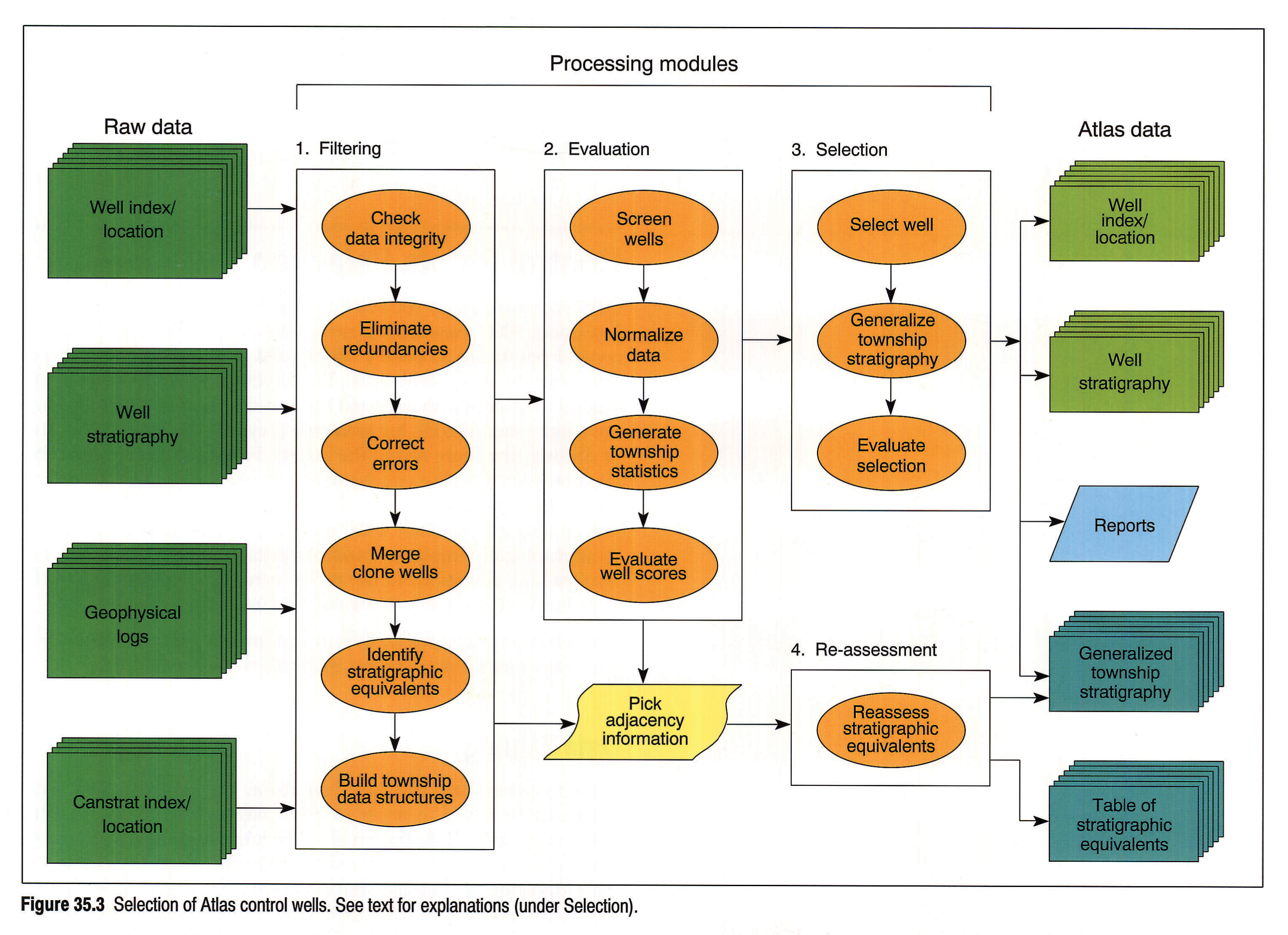
The selection of Atlas wells was performed by a program embracing all processing elements between the raw data and the Atlas database. The program consists of four major components: data filtering, data evaluation, well selection and final equivalents assessment (Fig. 35.3).
The data filtering module distils and organizes the raw data. It checks data integrity, eliminates redundant or unusable elements, corrects errors, evaluates and merges clone wells, identifies stratigraphic synonyms, and builds data structures. Lastly, it adds information on pick adjacency (overlay/underlay relations) and equivalency to reference storage.
The data evaluation module eliminates inferior wells (e.g., wells markedly too shallow for further consideration or with large gaps in its string of stratigraphic picks), normalizes the data to make the individual criteria comparable with one another, generates statistical characteristics of relevant well parameters, and assesses each well in the context of all other wells in a given township.
The selection module computes the total well merit as a weighted sum of well scores on each criterion, and selects the well with the highest merit. Stratigraphic data from the remaining wells in the host township are generalized by statistical parameters, and retained, together with a table of stratigraphic equivalents, as reference information. This module also generates a series of reports that allow a geologist to evaluate critically the results of selection. A choice of weights attached to each of the selection criteria, and several options on the evaluation function, provide mechanisms for human control of the process.
The program's final module is an error-correcting procedure that scans and refines the linkage data contained in reference storage. Reassessment of each township sequence and revision of the master equivalents table on the basis of corrected reference information completes the processing.
The analytical methods employed for optimization of well selection range from basic statistical tests and kernel estimations to more elaborate pattern recognition techniques. The latter are used for automating the most non-trivial and inexact parts of data assessment - the basic tasks of data filtering. When the program attempts to eliminate an inconsistency in the pick sequence, or to isolate stratigraphic equivalents, it is called upon to make a decision that requires some understanding of stratigraphic relations. Yet the diversity and complexity of the regional stratigraphy precludes the introduction of simplistic reference tables as the program's guide. Therefore, the program must extract stratigraphic knowledge directly from the data themselves, by examining and storing the adjacency relations between picks, and using the stored information, together with a few optimization algorithms and heuristic rules, to arrive at geologically sensible decisions. Exhaustive testing of program performance in these "fuzzy" tasks shows that the proportion of erroneous decisions rarely exceeds 5 percent. In such instances, prominent or obvious inconsistencies were corrected manually.
Atlas Database
The seemingly unavoidable dilemma in generating a stratigraphic database from disparate regional data sets can be loosely described in terms of Goedel's theorem - the database can be either consistent or complete, but not both. The diversity and subjectivity of geological information, together with the fluidity of stratigraphic interpretations and correlations, leave a database builder with only two (unattractive) options: 1) to re-arrange the data within some pervasive stratigraphic nomenclature, cull irrelevant information, and face potential complications in the database update, as new data and concepts clash with the established framework; or 2) to leave the data in their original state of disparity and completeness, and make accommodation for inevitable confusion in data retrieval, caused by the abundance of local stratigraphic names and the multiplicity of correlative relationships amongst numerous regions of distinct terminology.
Although aggravated by the degree of uncertainty that characterizes stratigraphic data, the consistency/completeness problem arises in dealing with any information that requires coding. Both the coding schemes and the encoded contents may differ widely between regions, and the question of whether to preserve local arrangements at the expense of database consistency, or to develop a general framework and tolerate certain losses of information, is basic in database generation.
The common solution to this problem is to design an overall coding order, and to relate it to the original local schemes with the help of reference tables. The disadvantage of this approach is that the relations between the local schemes themselves are built solidly into the database, and the latter must be re-assembled every time the relations change.
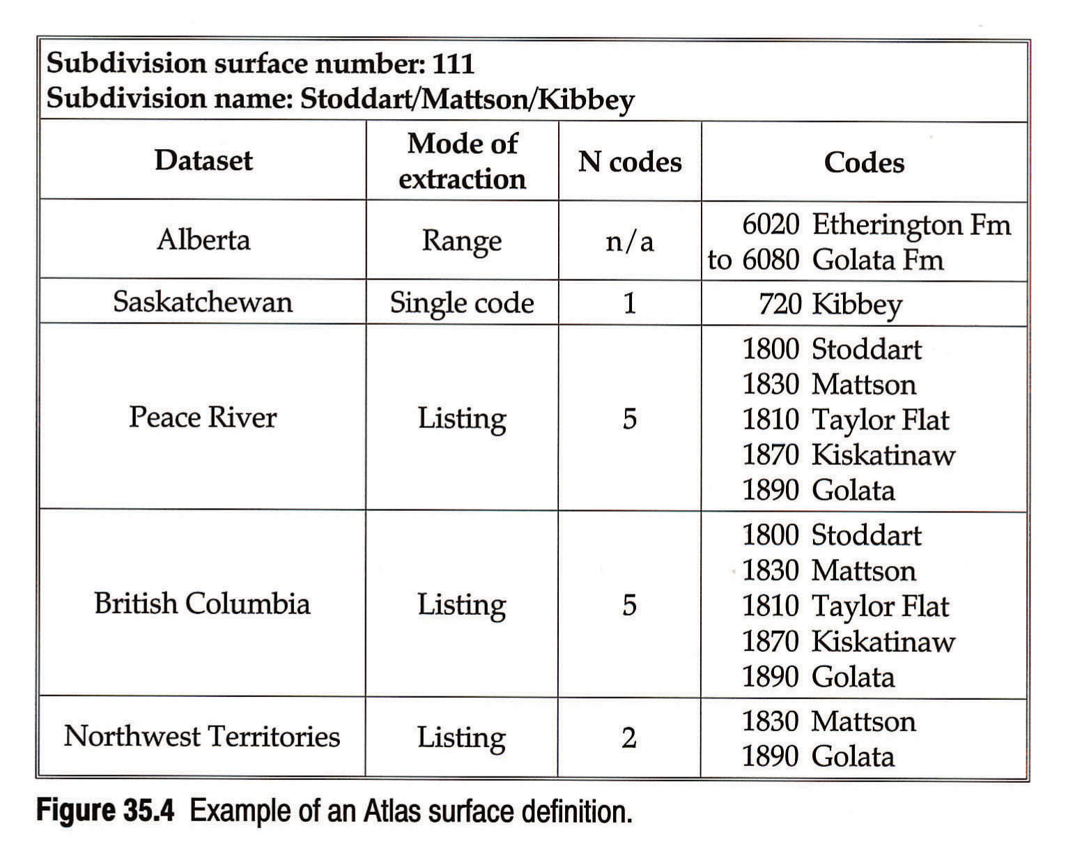
In the Atlas Database, the preference is given to completeness, that is, the regional coding arrangements are preserved, and all of the stratigraphic picks, whether they relate to Atlas stratigraphic slices or not, are retained. Thus, the data themselves bear little information as to their place within the Atlas stratigraphic framework. The slice stratigraphy and correlative relationships amongst regional nomenclatures are defined in the table of Atlas surfaces (Fig. 35.4), and the software links and integrates the data from regional data sets. Changing stratigraphic relationships, introducing a new stratigraphic subdivision, or redefining an existing surface all require revision of the table only. Every update and retrieval of data, on the other hand, is carried out within a virtual stratigraphic framework derived by a program from a current version of the table. This approach allows for both flexibility in stratigraphic analysis by chapter teams and ease of database maintenance.
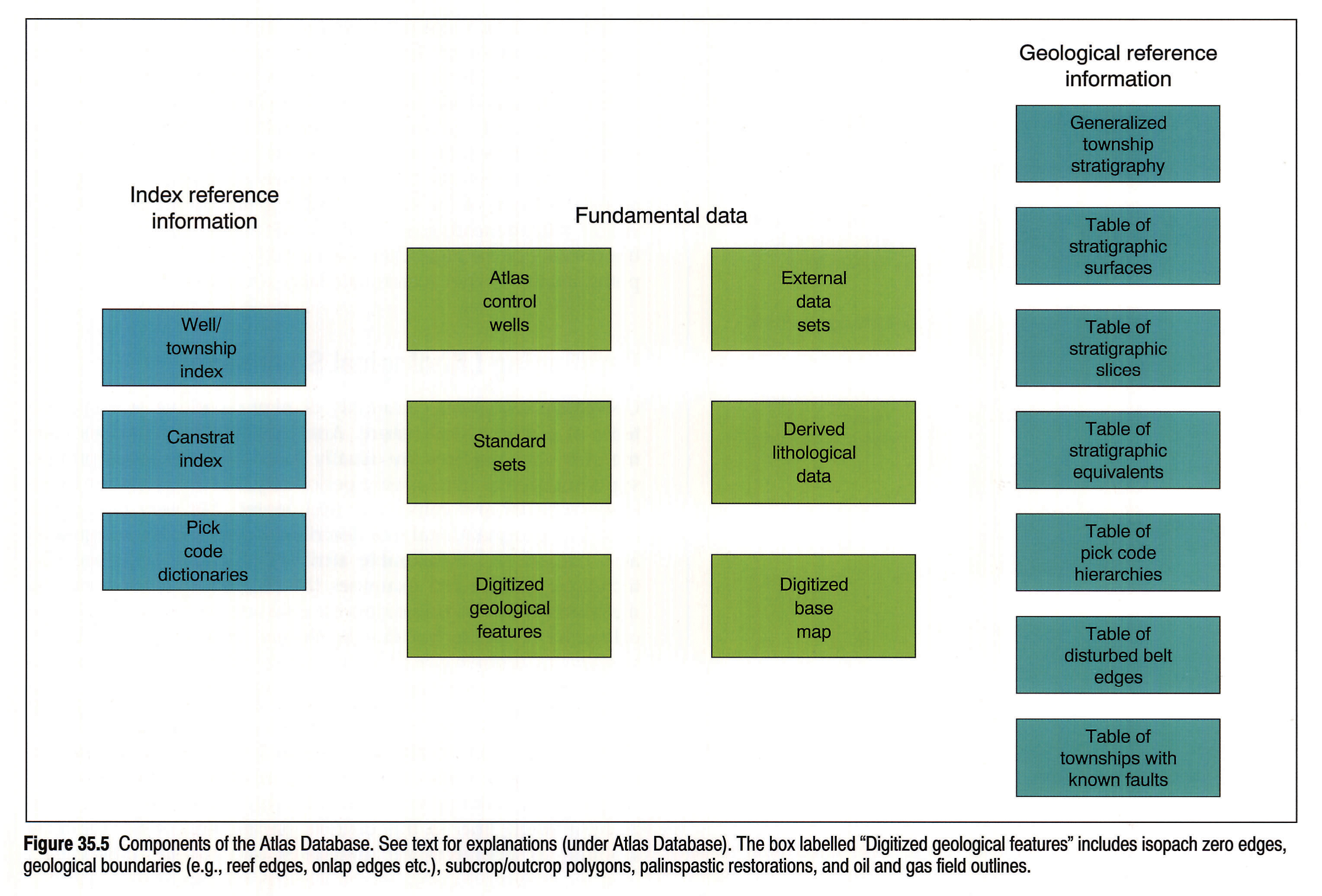
The Atlas database is depicted schematically in Fig. 35.5. The suite of Atlas control wells forms the core of the database, and represents the main source of map input data. It is subdivided into six regional data sets: Alberta, Saskatchewan, Manitoba, Peace River, British Columbia and the Northwest Territories. Each data set consists of two files: index and stratigraphy (see Fig. 35.3). The index information includes a unique well identifier, geographical coordinates, KB, total depth, Canstrat coverage, and a binary code indicating what significant geophysical logs are available for a given well. The stratigraphic data contain pick code, pick depth and, if applicable, the name of the Atlas reviewer, the date of revision and the type of update (e.g., confirmed depth, revised pick code, etc.).
The second large component of the database comprises external data sets submitted by chapter teams (Fig. 35.5). Generally, these contain wells in certain townships that are preferred over a given stratigraphic interval to the Atlas control wells. Notable exceptions are three extensive external data sets that include thousands of wells and cover large geographic areas: 1) near-surface coal exploration data in Alberta, provided by the Alberta Geological Survey; 2) Jurassic and Cretaceous data in Saskatchewan, donated by J.E. Christopher; and 3) Devonian Woodbend-Winterburn data, encompassing practically the entire basin. The Woodbend-Winterburn data set is exceptional, because it contains mostly Atlas wells in which the interval stratigraphy was completely redefined by the team. Because of the chapter team's conceptually distinct approach to stratigraphy, these data were introduced into the database as a separate data set.
An additional source of stratigraphic data is supplied by optimized sets of control picks. These data sets, denoted as Atlas "standard sets" (Fig. 35.5), are composed of picks selected (one per township) from a township population of like picks for a given stratigraphic surface. A non-parametric statistical method of kernel estimators (Hand, 1982) is employed to ensure that the elevation of a selected pick is optimally representative of a neighbourhood (township) cluster. Standard set data are invoked in townships where a corresponding pick in either Atlas or external wells is absent or obviously anomalous. These supplemental picks are particularly useful for mapping those horizons in the upper part of the stratigraphic succession that, because of casing or poor log quality, may be insufficiently covered by data from deep Atlas wells.
Generalized lithological data derived from the detailed and voluminous Canstrat Lithodata files (Fig. 35.5), and calibrated to the Atlas stratigraphy, are used for lithofacies characterization. The digitized base map and numerous files containing digitized geological features complete the fundamental data used for direct map input (Fig. 35.5).
The remaining files and tables comprise reference material and are invoked routinely by Atlas computer software operating on the database (Fig. 35.5). Index tables and pick code dictionaries help the programs to navigate through the complex network of regional data sets and stratigraphic nomenclatures. The geological tables supply the overall stratigraphic framework and some detailed geological knowledge required for data integration, organization and culling. The files containing generalized township information (Fig. 35.5) are used for well/neighbourhood cross-reference in data update and extractions. These files, generated in the process of control well selection (Fig. 35.3), contain a sequence of all stratigraphic markers encountered by at least one well in a township; for each marker, the data include the elevation mean and standard deviation, the number of wells in which the pick is recorded, and potential stratigraphic equivalents of the marker.
Data Maintenance
The Atlas database is maintained by a series of programs that perform all the operations related to data entry, update, retrieval and characterization. Even in reduced form, the data are too voluminous and the relationships too numerous for manual data processing. At each map iteration, the average number of data extraction specifications counts in the hundreds, and the number of contributors' data submissions (corrections and verifications) in the thousands. This volume of information, coupled with the diversity of stratigraphic relations, some inevitable overlap and conflict of information coming from different chapter teams, and the variety of formats in which the data circulate between the headquarters and the authors make automated processing the only practical vehicle to keep the database and data derivations orderly. The essential task of human assessment and verification of the results of data manipulation is achieved through exhaustive reports on operations and data changes generated by each program.
The most exacting operation in maintenance of the Atlas Database is its updating. A total of just over 150 000 stratigraphic data entries were processed by the system; approximately 45 000 of them revised data in Atlas control wells, and the remaining 105 000 entries related to the external data sets.
The data are introduced into the database in one of two ways: in a few cases by "block replacement", where the existing sequence of picks in a given Atlas well is totally removed and replaced by the new sequence of picks; and, much more commonly, by "integration", where some of the existing picks are preserved in the well record, provided that they do not contradict the new picks. To ensure the integrity of the data, the update program performs very extensive testing of every revision in the context of other well revisions, both previous and current, the overall well and township stratigraphy, and the reference tables. If ambiguous, inconsistent or contradictory revisions are attempted, the program itself validates or rejects data entries; it also has the capacity to optimize revisions, decide on the comparative validity of new and existing data, and generate replacement or deletion transactions that are implied but not stated explicitly by a contributor. Commonly only about 2 to 3 percent of data entries are rejected as irreconcilable. The update is performed in two steps: first, the program generates an update image and reports on potential problems; and then, only after the problems have been manually assessed and, if possible, rectified, is the actual revision of the database implemented.
Map Production
Atlas regional structure and isopach maps carry several layers of information (base map, well postings, contours, lithofacies areas, polygons and vectors depicting geological features; e.g., outcrops, zero edges). Each layer is in effect a separate map, but there is no scope here to enumerate in detail all of the procedures involved in their derivation and assembly. Only the contour and lithofacies maps, requiring the most elaborate processing and data analysis, are discussed.
Contour Maps
The contour maps were produced and refined through a continuous iterative process of map generation and data revision. At each iteration, maps were compiled at project headquarters and dispatched to chapter teams for evaluation, together with tables listing wells where pertinent data are missing or where existing picks are isolated as "potentially erroneous", to be manually verified and corrected. After the new data submitted by the teams were fed back into the database, a new generation of maps was produced and assessed. This process ensured gradual improvement in the quality of data and derived maps, while preserving, at each stage, the overall consistency and compatibility of maps from different stratigraphic slices.
The preliminary maps were generated by computer contouring software, without manual input. Compilation of the final maps, however, involved painstaking manual verification of the correspondence between computer-generated contours and control points, with consequent (considerable) adjustment of the contours. Maps reflecting very complexly differentiated surfaces, such as the Viking and Mannville isopachs, were compiled manually.
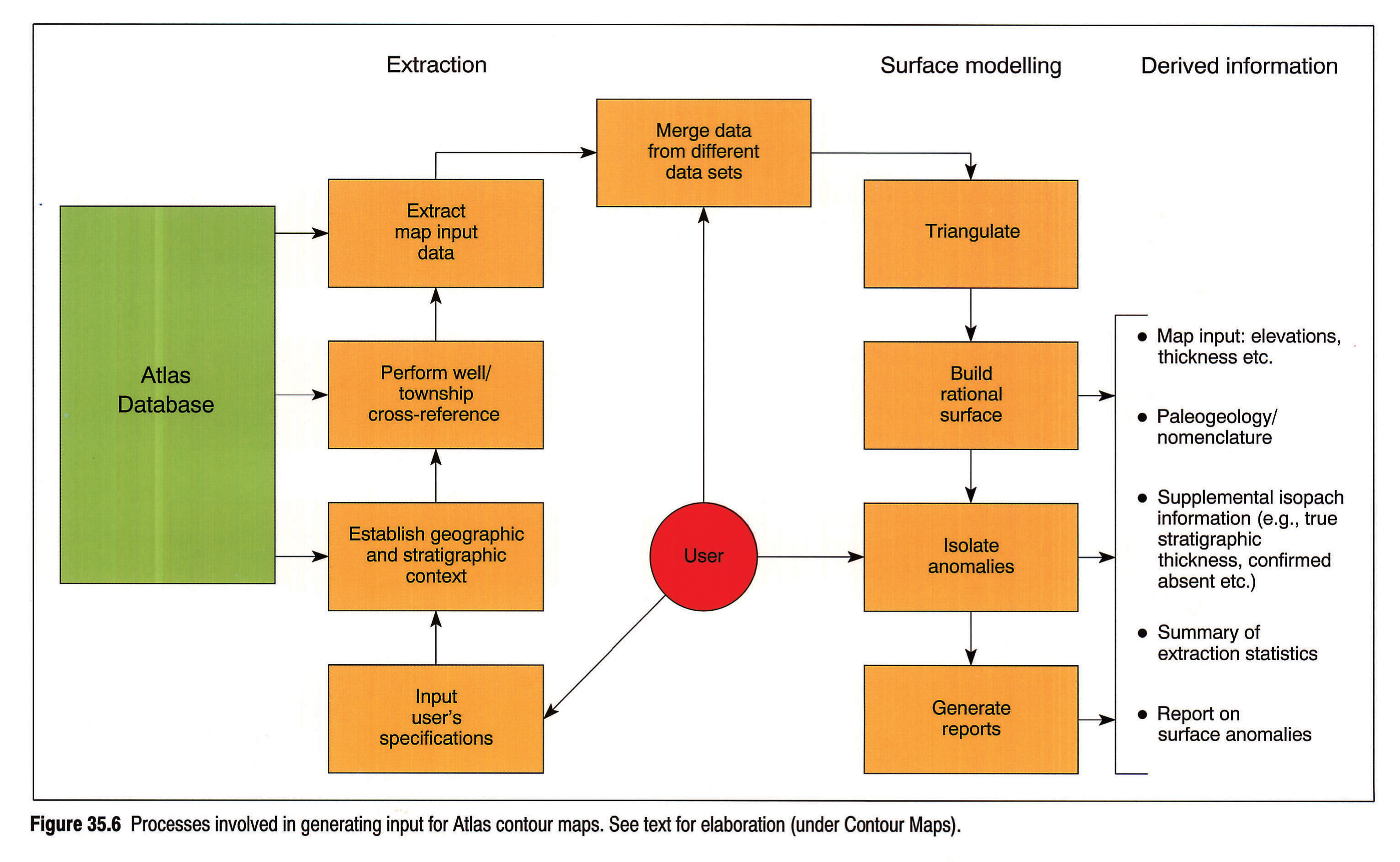
Generation of data input for contour maps consists of three main steps: data extraction, merging and analysis (Fig. 35.6). As with other components of Atlas data processing, the procedure is fully automated. The user specifies the integer code of required surface(s) (see Fig. 35.4), the desired output, and the order of data set precedence in data merge. In the extraction operations (Fig. 35.6), the programs themselves establish the geographic and stratigraphic relations between regional data sets, and perform a data search in the context of well and township stratigraphy. User's options include the search for stratigraphic equivalents of designated picks, the extraction and optimization of data defining isopach zero edges, and the splitting into paleogeology/nomenclature subsets.
Each source of stratigraphic information (control wells, external data sets and standard sets) is scrutinized separately, and yields its own file of pertinent records. The data merge (Fig. 35.6) involves selecting picks, one per township, from one of the three files. Preference is commonly given to an Atlas control well or an external well. The rejected records form a reserve of data to substitute, if necessary, for picks identified as erroneous by subsequent data analysis.
The final stage of data preparation is the isolation of anomalous points, with the help of the surface modelling technique developed for the project (Fig. 35.6). The procedure generates a triangulation of data points, and builds a generally "rational" surface from the data themselves, taking into account the natural roughness of a given surface. Each actual data point is then compared with its computed counterpart, and is designated as anomalous if the difference in values exceeds a certain user-specified magnitude. The anomalous wells are assembled into a table and referred to contributors for correction or verification. Built into the Atlas data processing software, the method constitutes an effective mechanism for both isolating and culling erroneous data, and highlighting anomalies of true geological origin.
Lithofacies Maps
The Atlas lithofacies maps are based on lithological information extracted from Canstrat Lithodata files, processed through a series of analytical procedures discussed under Data Analysis. One of the principal challenges proved to be the development of techniques and associated software to identify significant breaks in the lithology, and to match lithological breaks with log-based stratigraphic picks in the same vertical succession, in order to ensure that lithological characterization be properly calibrated to the Atlas stratigraphy. Files of derived Lithodata, generalized within stratigraphic intervals designated in Atlas control wells, provide data input for the lithofacies analysis and subsequent mapping.
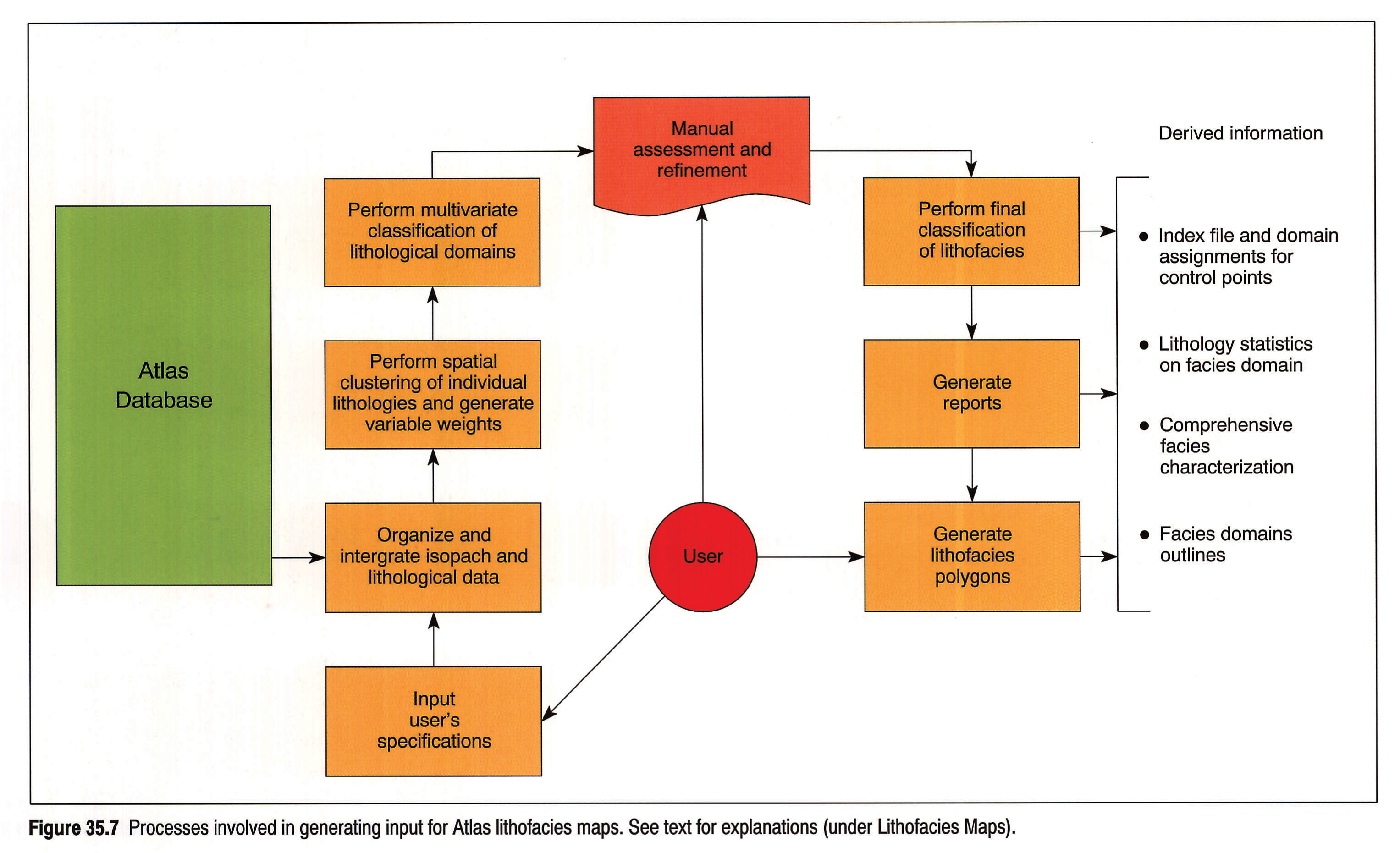
The operations involved in deriving lithofacies map input are illustrated in Figure 35.7. A program performs the spatial classification and characterization of lithological domains, with the assistance, if desired, of a geologist. At program initiation, the user is offered a choice of evaluation methods controlling the degree of map generalization. After the program has organized and integrated isopach and lithological data, and established linkage relations between neighbouring data points, it proceeds to consecutive evaluation and clustering of all individual lithologies contained within the designated stratigraphic interval. The degree of spatial separability of each lithology defines its weight in the subsequent multivariate classification of lithological domains (areas with optimally distinct percentage compositions). To facilitate visual assessment of classification results, domain assignments for control points of determined lithological affinity are transformed into domain outlines. Subsequent manual refinements may include selecting a different method of evaluation, adjusting variable weights, combining two or more domains, re-assigning individual data points, or smoothing out domain boundaries. After the final classification, the program generates a table of lithology statistics on facies domains and a report containing detailed lithofacies characteristics.
Data Analysis
The five analytical techniques presented here solve vastly different classes of problems and, consequently, use different means of data evaluation. Three belong to the class of pattern recognition problems: identification of stratigraphic equivalents, matching of lithological and stratigraphic data, and classification of lithofacies. Two are in the realm of numerical methods: isolation of surface anomalies and partitioning of lithological sequences. What the techniques have in common, however, is the general approach to data modelling, known as the geometrical method of computer data analysis (Devijver and Kittler, 1982). This approach concentrates on finding data representations and organizations, together with associated data structures and algorithms, in order to discover or highlight relationships within complex data sets. The underlying idea is that the best data models are the data themselves, and, given a suitable data representation as a general framework, an optimizing algorithm will draw out the natural order embedded in the data set.
Identification of Stratigraphic Equivalents
The problem of isolating stratigraphic synonyms is solved through the application of a graph-theoretic model for structural representation and transformation of stratigraphic data. The processing is performed on a township-by-township basis. The input is the record of stratigraphic picks in all wells located within a current township. The output is the complete township stratigraphic sequence, with indication of which markers are classified as stratigraphic synonyms. Since the technique has already been published (Shetsen and Mossop,1989), only the general approach to the problem is discussed here.
Recognition of stratigraphic equivalents is in essence the separation of a stratigraphic sequence into equivalence classes, mutually exclusive clusters of stratigraphic markers. Because of the inexact nature of interpreted subsurface information, the partition is fuzzy; that is, the classes do not have precise criteria of membership, but are defined by the grade of membership. Furthermore, the relation of equivalency is not transparent in a stratigraphic sequence that directly yields only the relation of pick adjacency. Therefore, the problem of recognizing equivalents amounts to finding a data representation and implementing algorithm that allow transformation from an observed crisp relation "marker A overlies marker B" to a fuzzy relation "marker B is likely to be an equivalent of marker C".
In the applied model, data are represented by the mathematical structure of a directed acyclic graph. The algorithm iteratively decomposes the graph into a collection of pairwise disjoint complete maximal subgraphs corresponding to the clusters of stratigraphic equivalents. In the trivial case where no synonymy is present, each cluster has only one member, and the number of clusters is equal to the number of defined picks. In the more general case, a cluster may contain several stratigraphic markers. Assignment to a given class ensures the maximal cohesiveness of the cluster. The average affinity of each marker to other markers defines its grade of membership. A pairwise measure of similarity is obtained as a function of the proximity of edges in a current graph, and the linkage data retained by the program from the preceding graphs. Thus, the effectiveness of the algorithm increases with the volume of processed stratigraphic data.
Isolation of Surface Anomalies
In this technique, a map surface is approximated by a triangulated regular region1, and is smoothed by the application of a converging surface envelope. The difference between the real and computed Z-values at each control point defines the grade of non-conformity, which can be visualized as a difference map. The points are classified as anomalous or non-anomalous simply by establishing some subjective threshold convenient for a current evaluation.
There are three data representations and associated data structures. Each control point is: 1) a node in the global triangulation network; 2) the centre of a polygon bounded by edges connecting all neighbours of the point in the network; and 3) an isolated node circumscribed by a triangle having three polygon neighbours of the point as its vertices. The first representation provides the regional framework for envelope construction; the second defines the neighbourhood for local evaluation of the surface; and the third allows a Z-value of the point to be interpolated from Z-values (either computed or real) at the vertices of the enclosing triangle. The algorithm iteratively transforms the actual map surface into an optimized smoothed surface, by building and evaluating a series of intermediate surfaces bounded by the gradually converging envelope. The estimating function minimizes the weighted average gradient of each point within its polygon, and maximizes the number of neighbouring points that retain their real Z-value. This maximization prevents the computed surface from becoming too smooth, and preserves the natural roughness of the map. Generally, between 50 and 75 percent of data points conform absolutely to the model surface.
Surfaces are constructed as follows. At each iteration, every data point has two Z-values, one of which is retained from the previous iteration, the other estimated currently from the vertices of the circumscribing triangle. The higher of the two values is assigned to the upper surface of the envelope, and the lower to the lower surface. After the envelope has been defined over the whole region, the procedure builds a current model from the three existing surfaces (the model surface generated at the previous iteration, and the current upper and lower surfaces of the envelope). Every point is assessed within its local neighbourhood at each of the three surfaces, and the Z-value from the surface with the optimal estimate is assigned to the current model surface. The procedure iterates until the envelope vanishes; that is, when the retained and interpolated Z-values of each point either become identical or fall within a small assigned range.
Testing has shown that this technique distinguishes well between rational variations in the map relief and the sharp changes that invariably result in large deviations of the model from the real surface. The algorithm isolates both the anomalies controlled by a single point and the anomalies produced by clusters of points, provided that the latter are expressed as tangible deflections in the surface. The technique does not require any a priori assumptions about the shape of the surface, and is generally robust. The edge effects, related mostly to ill-conditioned triangles, are minimal, and the stability of the algorithm is ensured by relatively simple computations that do not accumulate large rounding errors.
Partitioning Lithological Sequences
Geological sequences commonly display repetitive or cyclic patterns of a hierarchical nature. Analytical methods to detect and measure such patterns are usually based on some assumption of superimposed or overlapping periodicity. Yet the cycles are inherently irregular and commonly fragmented, but very rarely periodic. The computational tool described here treats the irregularity as a natural and measurable attribute of a data sequence. The technique detects and examines the changes in a succession of measurements, and transforms the data sequence into a hierarchical family of breaks, partitioning the succession into fractally homogeneous segments of different orders. Although developed for lithological data, it is applicable to any sequence of the time series measurements.
A succession of fluctuating data values can be viewed as a collection of aggregates reflecting a non-uniform, potentially hierarchical distribution of matter (called "curdling" by Mandelbrot, 1983), along a single line. In this context, partitioning of the sequence amounts to separating the aggregates, and, further, their groupings, by deriving the optimal set of end points. As several orders of curdling may be present in the succession, it is essental to find a suitable geometrical representation in order to highlight the hierarchical structures hidden in the data. The so-called "Devil's Staircase" (Mandelbrot, 1983) suggests a geometrical model for transforming the irregularity inherent in time series measurements into a more uniform and meaningful pattern of variations.
In the case of lithological sequences, interval measurements of a lithological variable (e.g., silt content or anhydrite content) are converted, from the bottom up, into cumulative values that form a continuous nondecreasing curve composed of many short straight-line segments with different gradients. Joints between the pieces of the cumulative graph can be graded by how critical they are in the overall shape of the curve, or, in other words, how sharp the curve is at these points. Joints of the first order control the most profound changes in the general slope of the curve; joints of the second order segregate lesser variations of the gradient within the segments bound by the first-order joints, and so on. Obviously, the gradients in the immediate vicinity of a joint give no indication of its order; the latter can be evaluated only in the context of the whole curve. In graphs of differentiable functions without local extrema, the points optimally separating the segments with different gradients are those with the maximum curvature on the concave upward or concave downward parts of the graph. Although not applicable directly, this measure can be approximated for optimal partitioning of nondecreasing irregular curves.
Decomposition of a sequence is attained through a series of geometrical constructions performed by an iterative algorithm. Each construction builds an envelope around the curve or a part of the curve, in the manner described above under Isolation of Surface Anomalies. The computation continues, and the envelope expands until it "submerges" all joints on the curve, except for those that refuse to be "drowned", namely, those points that control the overall concavity of a current segment. From these joints, the optimal points are selected, one for each concave upward or concave downward part of a curve. They form a set of end points subdividing the curve into segments of the same order. Each point is characterized by its order, the direction of concavity (sign), and the estimated area of the envelope region controlled by this point (magnitude). Each of the several curves resulting from the subdivision are subdivided again, yielding still smaller curve segments with a set of end points of the next order. This process continues until the segments are reduced to the basic linear pieces of the original curve.
A hierarchical family of end points, or breaks, stratifies the succession. The strata are also hierarchical, in the sense that, except for the basic intervals, each layer is an aggregate of lesser layers. Smaller sequences reveal three to four levels of stratification, and more complex successions may contain up to eight orders of aggregation. The most obvious yield from hierarchical sequence partitioning is the framework it provides for generalizing interval characteristics at different scales. This in turn facilitates classification and correlation of sequence cycles. Another product of the process is the breaks themselves, which are, in essence, scaling sets of points, of the nature of fractal dusts. Their distribution, order, sign and magnitude provide additional quantitative information for investigating and modelling sequence dynamics.
Matching of Lithological and Stratigraphic Data
Calibration of well stratigraphy to variations in lithological sequence; that is, attaining some optimal correspondence between the two data successions, can be viewed as mapping a sequence of stratigraphic markers into a sequence of lithological breaks under certain constraints. The first constraint is that a sequence of log-based stratigraphic picks is generally fixed, and so the change in the position of stratigraphic markers should be minimal. The second constraint is imposed by the condition that each stratigraphic marker can be mapped only into that part of the lithological succession that is bounded by the two adjacent markers.
The matching algorithm, although computationally intensive, is conceptually straightforward. A stratigraphic sequence is designated as a system of joined blocks - stratigraphic intervals characterized by their position and their state. The position is defined by the depths of the top and bottom stratigraphic picks marking off the interval, and the state is determined by a number of parameters derived from the lithological data. Among these parameters are the percentage composition and the vertical variability of individual lithologies (e.g., shale, limestone, anhydrite etc.), lithological homogeneity of the interval, the difference in lithological characteristics between adjacent intervals, and the orders and magnitudes of lithological breaks contained within a given segment. The original stratigraphic sequence induces the initial states. Modification of the position of a block changes the states of this block and its neighbours, increasing or decreasing their stabilities. The goal of processing is to maximize the overall stability of the system.
Stability is measured by a function that minimizes the change in the position of a block and maximizes a favourable modification of its state. What constitutes a favourable modification is defined by the initial state of a block in the context of adjacent blocks. For example, homogeneity is maximized in a generally homogeneous block with less homogeneous neighbours, and vertical variability is emphasized in a highly interbedded block adjacent to less interbedded blocks. Mapping the joint of two blocks into a lithological break may increase or decrease their stabilities, depending on whether or not the sign and magnitude of the break correspond to other parameters. Thus, each state is evaluated by the inner product of the vector of state parameters and the vector of weights characteristic for a given block. The algorithm performs sequential adjustment of blocks, selecting at each step the most homogeneous unit not already processed. All possible states within the permissible range of positions are assessed, and the position producing the highest stability is accepted. After each adjustment, the states of all blocks are revised.
Testing and subsequent application of the technique to lithological data have shown that the effectiveness of the algorithm depends mostly on how inclusive is the string of stratigraphic picks. The best results are achieved for wells with a comprehensive stratigraphic record. Successions with incomplete stratigraphic documentation are more likely to contain matching errors.
Classification of Lithofacies
Spatial classification of lithofacies is based on a graph-theoretic model of clustering that brings out internal data structure by connecting close elements into minimal spanning trees (Kandel, 1982). For the sake of processing efficiency, the clustering is performed on a triangulated network of data points; that is, each point is compared with a limited group of neighbours defined by the triangulation. The algorithm is an iterative procedure using the agglomerative approach, so that a final set of trees is formed by successively merging smaller subtrees defined at the previous stages. At each iteration, the procedure generates a current triangulation network with each subtree forming a single node. After several iterations, each node becomes a hierarchy with several levels of agglomeration. In some instances, the program explores this structure to determine the degree of similarity between two trees. Processing stops when dissimilarity between nodes exceeds a certain threshold.
Each node in the network is defined by some characteristic value. At the initial stage, it is simply either the percentage of an individual lithology, in the case of one variable, or a weighted average of several percentages, in multivariate classification. The weight reflects the discriminating power of a given lithological variable, and is generated by the program, although a mechanism for manual adjustment is available. Each edge is characterized by a cost defined by a pairwise measure of similarity between two connected nodes. By user's choice, the similarity is computed either as a functional of the distance (difference in values) between two vertices, or as the general weighted distance that takes into account not only the similarity of characteristic values but also the structure of the nodes. The latter measure induces larger spanning trees, and, consequently, more broadly defined facies classes.
Construction of a current set of minimal spanning trees starts with computing the cost of each edge, and examining the edges in order of decreasing cost. If one of the vertices is connected, the edge is joined to an existing tree; otherwise, the edge initiates a new tree. After all edges have been processed, each tree is assigned a characteristic value computed as a weighted mean of values at the vertices. The weights are determined by the normalized average similarity of the nodes and their neighbours. In this way, the influence of extreme members on the characteristic value of the cluster is minimized.
The procedure consists of four steps. 1) The first construction produces, for each lithological variable, an initial set of clusters by means of simple comparison of point-to-point similarity. The number of clusters and the within-class/between-class variability define the weight attached to a given lithology in further processing. 2) Through a series of constructions, neighbouring nodes (trees) are merged until they form the minimal set under a subjectively defined threshold. 3) The resulting set of nodes is composed into a graph so that only those nodes that are not immediate neighbours are connected. These nodes are merged using the basic clumping technique of clustering, until their similarity is less than the assigned threshold. 4) The last step includes interactive consultation with the user, and, if required, an adjustment of generated classes (the derived groupings of points). Generating class descriptions for the full set of lithological characteristics completes the processing.
Discussion
Atlas software was developed pragmatically, to resolve specific data processing issues. However, all such issues originally sprang from fundamental geological questions and all processing was targeted to the production of reliable geological maps. Although over 80 percent of the development effort was devoted to managing subsurface data and distilling its essence (the last 20 percent being expended on the final contouring and lithofacies depictions), the ultimate test of the Atlas processing must nonetheless be the maps themselves, their integrity and utility, and the veracity of the associated digital database.
Acknowledgements
Our most heartfelt gratitude is extended to Project Technician Kelly Roberts, who for upwards of five years expedited all elements of Atlas data entry and plotting - tens of thousands of records and hundreds and hundreds of map plots - always in good humour and always with stunning efficiency. She was ably assisted during peak-flow periods by Parminder Lytviak and Leslie Henkelman. Barry Fields was most conscientious and helpful in keeping the plotters running. Sheila Stewart provided sound technical help during 1989/90, and Joe Olic skillfully handled the bulk of the digitizing for Atlas plots (1990/91). All are gratefully acknowledged and thanked. Special thanks are reserved for Don McPhee, for his technical help in 1991/92, but more so for his moral support during the final two years of the project.
Output from the Atlas electronic system was processed using AGSSYS, an excellent cartographic system developed and maintained in-house by Andre Lytviak and the Alberta Geological Survey computing group. In direct support of the project, Mr. Lytviak set cartographic images and transferred them for final graphics processing. As head of the AGS computing group, he also provided invaluable support and hands-on help in a wide range of project needs in cartographic and graphics hardware and software. We are most grateful to him. Staff in the Alberta Research Council Computing Department are also thanked for their cooperation and for accommodating a lot of late-night computing, at vastly reduced CPU costs.
This manuscript benefitted from the thoughtful review and editing of Jim Dixon. Figures were digitally compiled by Jim Matthie.
Finally, we wish to thank all of the staff and management of the Alberta Research Council, and the Project Sponsors, who supported the development of the Atlas data processing system, both in concept and in fact.
References
- Devijver, P. A. and Kittler, J. 1982. Pattern Recognition: A Statistical Approach. London, Prentice/Hall International. 441 p.
- Hand D.J. 1982. Kernel Discriminant Analysis. Biometric Unit, Institute of Psychiatry, London University, England. Published by Research Studies Press. 253 p.
- Kandel, A. 1982. Fuzzy Techniques in Pattern Recognition. Florida State University, Wiley-Interscience. 356 p.
- Mandelbrot, B. B. 1983. The Fractal Geometry of Nature. International Business Machines Thomas J. Watson Research Centre, New York, W.H. Freeman and Company. 468 p.
- Renka, R. J. 1984. Algorithm 624. Triangulation and interpolation at arbitrarily distributed points in the plane. Association for Computing Machinery Transactions on Mathematical Software, v. 10, p. 440-442.
- Shetsen, I. and Mossop, G.D. 1989. Recognition of stratigraphic equivalents using a graph-theoretic approach, for the Geological Atlas of the Western Canada Sedimentary Basin. In: Statistical Applications in the Earth Sciences. F.P. Agterberg and G.F. Bonham-Carter (eds.). Geological Survey of Canada, Paper 89-9, p. 447-458.